• Introduction
• Model Experiment
• Advection Using Real Wind Data
• Conclusion
• References

FIGURES

• Figure 1
• Figure 2
• Figure 3
• Figure 4
• Figure 5
• Figure 6a - 6b

Introduction

Dynamical processes of transport and mixing around the wintertime stratospheric polar vortex have been examined in connection with the Antarctic ozone hole A transport barrier exists at the edge of the polar vortex and air within the vortex is isolated from outside. Studies on isentropic trajectories by using analyzed winds (Bowman 1993) and three dimensional models (Pierce and Fairlie 1993) showed that chaotic mixing occurs inside and outside of the vortex, respectively, based on the exponential growth of material contours and the patterns of stretching and folding.

Pierrehumbert (1991) applied the concept of chaotic mixing to geophysical flows; he investigated a planetary wave motion with a small periodic perturbation in a two-dimensional channel domain and showed the evidence of chaotic mixing in the flow. Mixing in two-dimensional nondivergent flows has been studied in relation with Hamiltonian dynamics for fluid particles.

In this study, the stratospheric polar vortex is idealized as a solution with quasi-periodic time dependence of a nondivergent barotropic model, and horizontal mixing around the vortex is investigated. The time periodicity enables us to use the same kind of analysis methods as in the kinematical studies of Hamiltonian dynamics. The flow field in our model has dynamical consistency because it is obtained in a direct numerical simulation of a full dynamical equation more akin to the atmosphere than previous kinematical models. In addition, the mixing process in the quasi-periodic flow is compared with that in a more realistic aperiodic flow of similar pattern which is obtained in the same model.

In the flows of our model, eastward propagating planetary waves generated through barotropic instability are dominant. The situation is close to that in the upper stratosphere of the southern hemisphere where the 4-day wave is often observed. The 4-day wave appears in the upper stratosphere in winter (Venne and Stanford 1979), more evidently in the southern hemisphere than in the northern hemisphere. It is dominated by zonal wavenumbers from 1 to 4, traveling eastward with the same phase speed. Observational and theoretical studies are summarized in Allen et al. (1997), and Manney et al. (1998). Relevance of the results in the model experiment to the real atmosphere is investigated using the same methods on isentropic surfaces.

Model Experiment

Model

A model of a two-dimensional nondivergent flow on a rotating sphere with forcing and dissipation is considered following Ishioka and Yoden (1995). The system is governed by a vorticity equation:

where q is the PV (or, the absolute vorticity in this case), and over-bar denotes zonal mean. The first term on the right hand side is a relaxation term to a prescribed zonally symmetric forcing defined below. with the relaxation time of ± = 10 days. The second term is an artificial small viscosity with ? = 6.43 x 10⁴ m² s^-1.

A spectral model with T85 truncation and the 4th-order Runge-Kutta method is used for time integrations with a time increment of 1/80 day. We use the analytic form of the forcing originally introduced by Hartmann (1983):

where U, B, and Æ₀ are parameters characterizing the polar-night jet; U is a measure of intensity of the jet, B its width, and Æ₀ its position. It is converted to forcing of PV in the vorticity equation.

We use two parameter sets, (U, Æ₀, B) = (180 m s^-1, 50°, 15°) and (180 m s^-1, 50°, 10°) . While these parameter sets are close to each other, the solutions are categorized into different regimes (Ishioka and Yoden 1995): the former parameter set gives a quasi-periodic solution, and the latter gives an aperiodic one. After the initial transient period, the flow settles into a state in which the forcing to intensify the unstable jet and the disturbances growing from the barotropic instability are balanced. We investigate the flow after 1000-day integration. And trajectories are computed simultaneously with the time integration of the flow field.

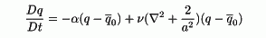
Finite-time Lyapunov Exponents

Finite-time Lyapunov exponent gives the exponential growth rate of the distance between two nearby trajectories. It depends on initial position and evaluation time. Figure 1 shows the spatial distributions of the largest finite-time Lyapunov exponents for the quasi-periodic solution (a,b) and the aperiodic solution (c,d) for two evaluation times of Ä=2 and 90 days. Calculations are done on every 2° x 2° grid in the latitudes of Æ > 20° with two small perturbations of angular length of 10^-6rad in longitudinal and latitudinal directions. Linear deformation effect due to horizontal shear appears in the both results of Ä=2 days (a,c) because of the short evaluation time. Low value is seen on a ring corresponding to the edge of the polar vortex. High value is seen in the both flanks of the jet, particularly in the equator side. The effect by chaotic behavior of the particles is not clear at this stage. For longer time intervals, the exponent shows stronger dependence on the initial position, since Lagrangian behavior is chaotic. In the quasi-periodic flow, the ring of low value is well identified even for Ä=90 days at the edge of the polar vortex (b). The edge of the polar vortex is less evident (d) in the aperiodic solution, but the value inside is lower than outside, which is consistent with previous studies (e.g. Bowman 1993; Bowman and Chen 1994). Spatial distributions for the both solutions show large inhomogeneity inside the polar vortex. A large triangular region with round corners in which the value is very low is seen inside the vortex. The region is still discernible in the both solutions even Ä=90 days. In addition, a croissant-shape region with low exponent is also seen between the triangular region and the vortex edge, particularly in the quasi-periodic solution.

Fig.1 Distributions of the largest finite-time Lyapunov exponent on all grid of 2 degrees for the quasi-periodic solution (a,b) and the aperiodic solution (c,d).

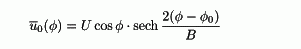
Poincare Sections in the Quasi-periodic Flow

In the quasi-periodic flow, Poincare sections are available in this co-rotating frame with the vortex Trajectories of several particles are calculated for a long integration time, and the positions at every one vacillation cycle are all plotted on one figure. Figure 2 shows the Poincare sections computed for 1000 vacillation cycles with 12 particles initially put outside the polar vortex (a), and 19 particles inside the vortex (b). Regions where particles have chaotic, irregular trajectories are the chaotic mixing regions, while regular trajectories are seen in the regions of invariant tori where the fluid is not mixed but only stirred. Outside the polar vortex (a), chaotic mixing region is recognized in midlatitudes. Closed loops of dashed line found at the both sides of the mixing zone are invariant tori. The one inside the mixing zone (blue, dashed line) coinsides with steep PV gradient at the polar vortex edge. One more torus of croissant shape is also found just outside of the edge (red line). Another chaotic mixing region is found inside the polar vortex (b) with more complicated structure of invariant tori; (1) central region of the polar vortex (green, solid loop), (2) three ``islands'' surrounding the central region, which are identified with three red loops, and (3) four thin islands just outside the three islands. These are transport barriers of different type from the polar vortex edge which are not related to any steep PV gradient.

Fig.2 Poincare section for the quasi-periodic solution. Initial 12 points are located outside the vortex (a) and 19 points are inside (b).

Particle Advections in the Aperiodic Flow

We make circles with a radius of 0.05 rad centered on the points at which the finite-time Lyapunov exponent for Ä=2 days is highest inside and outside of the vortex, respectively. Initially we put 10⁴ particles randomly in the circle and computed their trajectories for 90 days in order to have fundamental pictures of the mixing process.

Results for the aperiodic solution are shown in Fig.3. The particles outside the vortex (red) are well-mixed in 90 days. At first, particles are stretched out to west and east by the meridional shear of the jet. They become distributed on a thin line element surrounding the polar vortex. At the same time, the element is distorted and folded at several places. Such stretching and folding processes are repeated and the layered structures of the particles are made. Combined with the positive Lyapunov exponents, chaotic mixing dominates the large-scale mixing process. Transport barriers exist at the both boundaries of the chaotic mixing zone, just on the vortex edge that is defined as the largest meridional gradient of PV at each longitude. While planetary-wave breaking events make a small amount of the particles go outside of the vortex for 90 days, there are no incoming particles from outside during the period.

Particles inside the polar vortex are also mixed in a similar way (blue). But they do not spread all over the vortex inside. Several empty regions exist even at t=90 days; the core of the vortex, three small "island" regions surround the core region, and a croissant-shape region near the vortex edge. The method of Poincare section cannot be used for aperiodic solutions, but some features obtained in Fig.2 for the quasi-periodic solution have correspondence with empty regions found in Fig.3; isolation of the central region of the polar vortex, the croissant-shape region, and the three islands surrounding the central region.

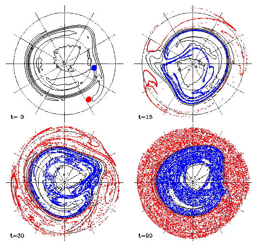
Fig.3 Advection of 10000 particles for 90 days in the aperiodic solution.

Advection Using Real Wind Data

Data

In order to investigate the relevence of the structure found in the model experiment to the real atmosphere, UKMO Assimilated Data is used to advection experiments on isentropic surfaces in the wintertime upper stratosphere. The data contain fields of temperature, geopotential height, and wind components on the levels from 1000hPa to 0.316 hPa on a 3.75° x 2.5° grid.

Horizontal wind data are interpolated on isentropic surfaces and linearly interpolated in time. The data on isentropic surfaces are expanded to spherical harmonic function and wind velocity on arbitral point is calculated by reverse transformation of the spectrum.

The wintertime upper stratosphere in the southern hemisphere is examined, where the 4-day wave caused by barotropic instability of the polar-night jet is dominant and turbulent mixing due to breakings of the planetary waves propagating upward from the troposphere is considerably weak.

Hovmoller Diagrams

Figure 4 is time-longitude sections at 1800K and 72°S of wave 1 in PV, showing moving component by substracting 20-day running mean. Generally, eastward-propagating wave with period of 3-4 days, called the 4-day wave is dominant in wintertime upper stratosphere. It is dominated by zonal wavenumbers from 1 to 4, traveling eastward with the same phase speed.

Large wave amplitude propagating eastward with period of 3-4 days is seen in 1999 (top), especially in mid-winter. Calculations below are all started at Jul 7. We compared results in 1999 with those in 1992 (bottom), in which the amplitude is weakest of all the past available data.

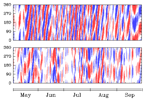
Fig.4 Time-longitude sections at 1800K and 72S of wave 1 in PV, showing moving component by substracting 20-day running mean, in 1999 (top) and 1992 (bottom).

Finite-time Lyapunov Exponents

Finite-time Lyapunov Exponents are calculated with the evaluation time of Ä=10 days as shown in Fig.5, with the snap shot of PV at 1800K on Jul. 7. The edge of the polar vortex is on 45-55°S. Distribution of high exponents outside the polar vortex show the evidence of strong mixing. Very low exponents at the edge of the vortex suggest that transport barrier is formed there. Inside the vortex, we can see the differences between the two results. Relatively high region is on 60-70°S in 1999 (top), while almost whole region inside the vortex is covered with low exponents in 1992 (bottom). The high region in 1999 corresponds the region of strong signal of the 4-day wave.

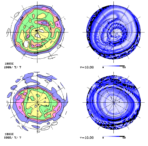
Fig.5 Snap shot of PV on 1800K on Jul 7 in 1999/1992 (left). Finite-time Lyapunov Exponents calculated from Jul.7 with the evaluation time of 10 days (right).

Particle Advections

Dispersion of lots of particles placed in an limited area is computed on the isentropic surface. We select five points at which the finite-time Lyapunov exponent for Ä=10 is highest and lowest, respectively, inside the vortex. Initially we put 1000 particles randomly in the circle centered on the points with a radius of 0.05 rad, and calculated the advections of the particles. Figure 6 shows the results in 1999 (top) and in 1992 (bottom). Warm colors denote the points of high exponents, and cold colors denote low. At first, particles are stretched out to a thin line element and, after that, the element is distorted and folded. Stretching and folding processes are repeated and particles are mixed with surrounding as seen in the model experiment. However, well-mixed region is limited to a finite area near the 70° and the particles in the other region keep their identities even after 20-day advection. In 1992, on the other hand, air inside the polar vortex rotate around the pole like a rigid body. Only particles near the edge of the vortex is stretched by the meridional shear of the jet, but not mixed after 20-day advection.

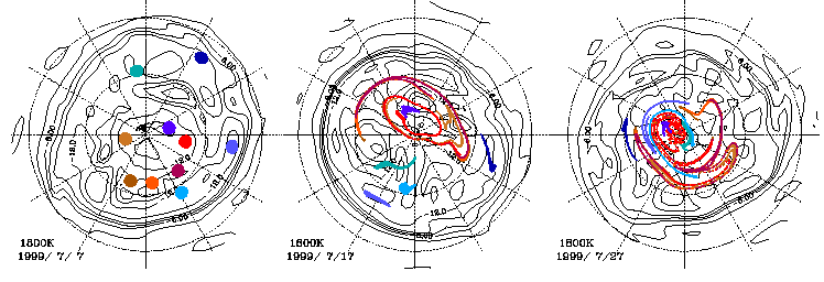
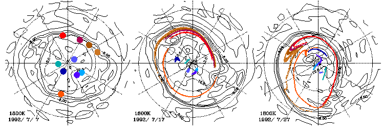
Fig.6 Advections on 1800K of 1000 particles from five points at which the finite-time Lyapunov exponent is highest and lowest, respectively. Calculations start Jul. 7 1999 (top) and in 1992 (bottom).

Conclusion

Chaotic mixing in dynamically consistent flows obtained as numerical solutions of the barotropic vorticity equation was investigated. The barotropic model is a forced-dissipative system which simulates an idealized polar vortex, especially in the wintertime upper stratosphere. A typical example of chaotic mixing is obtained for the quasi-periodic flow. Effective, irreversible mixing occurs through stretching and folding process outside of the polar vortex, and inside as well. The transport barriers are identified precisely as invariant tori in the Poincare sections. In addition to the barrier associated with steep potential vorticity gradients on the edge of the polar vortex, transport barriers which is not related to the potential vorticity gradient is found inside the polar vortex. Furthermore, it is revealed that the structure obtained in the quasi-periodic flow is relevant to flows that are weakly aperiodic.

Relevance of the transport barrier found in the model experiment to the real atmosphere was investigated using horizontal wind data on isentropic surfaces. We examined in the wintertime upper stratosphere in the southern hemisphere, where irregularity of the flow is considerably weak. When the 4-day wave has a large amplitude, distributions of finite-time Lyapunov exponents show a large inhomogeneity inside the polar vortex. Effective mixing through stretching and folding process is seen on about 60-70°, where the Lyapunov exponent is high. But particles are not mixed in the other region. When the wave is not seen, on the other hand, Calculation of finite-time Lyapunov exponents and particle advections inside the vortex suggest that mixing does not occur.

References

Allen, D. R., and J. L. Stanford, L. S. Elson, E. F. Fishbein, L. Froidevaux, and J. W. Waters, 1997: The 4-day wave as observed from the Upper Atmosphere Research Satellite Microwave Limb Sounder. J. Atmos. Sci. 54 420--434.

Bowman, K. P., 1993: Large-scale isentropic mixing properties of the Antarctic polar vortex from analyzed winds. J. Geophys. Res. 98 23013--23027.

Hartmann, D. L., 1983: Barotropic instability of the polar night jet stream. J. Atmos. Sci. 40 817--835.

Ishioka, K., and S. Yoden, 1995: Non-linear aspects of a barotropically unstable polar vortex in a forced-dissipative system: Flow regimes and tracer transport. J. Meteor. Soc. Japan 73 201--212.

Manney, G. L., Y. J. Orsolini, H. C. Pumphrey, and A. E. Roche, 1998: The 4-day wave and transport of UARS tracers in the Austral polar vortex. J. Atmos. Sci. 55 3456--3470.

Mizuta, R., and S. Yoden, 2000: Chaotic mixing and transport barriers in an idealized stratospheric polar vortex. J. Atmos. Sci., Submitted.

Pierce, R. B., and T. D. Fairlie, 1993: Chaotic advection in the stratosphere: Implications for the dispersal of chemically perturbed air from the polar vortex. J. Geophys. Res. 98 18589--18595.

Pierrehumbert, R. T., 1991: Large-scale horizontal mixing in planetary atmospheres. Phys. Fluids A3 1250--1260.

Venne, D. E., and J. L. Stanford, 1979: Observation of a 4-day temperature wave in the polar winter stratosphere. J. Atmos. Sci. 36 2016--2019.