Figure 1. Percent contribution of stratospheric ozone(%) at the surface
and 500 hPa for January and July.
Center for Climate System Research, University of Tokyo, Meguro-ku, Tokyo, 153-8904, Japan
Frontier Research System for Global Change, Yokohama-shi, Kanagawa, Japan
FIGURES
Abstract
1. Introduction
Tropospheric ozone is not only a principal green house effect
gas, but also the most important chemical s. Understanding of
present global distribution and budget of tropospheric ozone is
very important for future prediction of atmospheric environment
and climate. Stratospheric ozone is one of possible source of
tropospheric ozone. Contribution of stratospheric ozone to the
global budget of tropospheric ozone is, however, still uncertain.
In this study, stratospheric effect on the distribution and budget
of tropospheric ozone is analyzed using a 3D chemical model.
2. Model overview
The model used in this study has been developed by using the Center
for Climate System Research/National Institute for Environmental
Studies(CCSR/NIES) AGCM. This model is aimed at studying the global
distribution and budget of tropospheric ozone and its precursors,
and radiative effect of tropospheric ozone. The horizontal resolution
is T21(5.6ox5.6o) with 32 layers in the vertical from the surface up to about
40 km altitude. In the present configuration of the model, the
chemical component of the model predicts the concentration of
24 chemical species between the surface and approximately 20 km
altitude, including 52 chemical reactions and 11 photolytic reactions.
In this study, only ethane and ethene are considered as NMHCs
trace gas. The model, however, can represent background chemistry
of the troposphere. More detailed chemistry including biogenic
NMHCs is now being implemented. The model also includes surface
emission and wet/dry deposition. Surface emission data are mainly
taken from Olivier et al., 1996. Detailed description will be discussed in Sudo et al.,(to be submitted).
3. Ozone contribution from the stratosphere
Figure 1 shows the percent contribution of stratospheric ozone
to the tropospheric ozone distribution at the surface and 500
hPa for January and July.
Figure 1. Percent contribution of stratospheric ozone(%) at the surface
and 500 hPa for January and July.
Surface contribution is greater than 50% in the mid-high latitude
in winter time and generally smaller than 10% in the polluted
region in summer time, reflecting strong photochemical production
of ozone. At 500 hPa altitude, contribution in the tropical region
is small throughout a year because of intensive and deep convection,
short life time of ozone associated with high humidity, and ozone
chemical production due to lightning NOx and biomass burning emission.
Figure 2 shows zonal averaged ozone contribution from the stratosphere.
The similar seasonal variation as Figure 1 is seen.

Figure 2. Zonal averaged percent contribution of stratospheric ozone(%)
for January, April, July, and October.
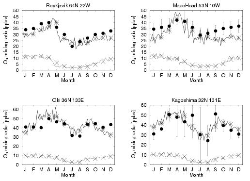
Figure 3 indicates the effect of stratospheric ozone on seasonality of surface ozone concentration. Ozone from the stratosphere does not seem to control seasonality of surface ozone in these selected sites.

Figure 3. Observed and calculated surface ozone seasonal variation for
4 selected remote sites (ppbv). (circles; observations, stars
and solid lines; model, cross and dashed lines; originated in
the stratosphere.
Tropospheric ozone budget in the model is seen in Table 1. Stratospheric ozone influx is relatively small compared to chemical production in the troposphere. The value of 636 TgO3/yr is within a range suggested in recent literatures(typically 400-1000 TgO3/yr).
NH
SH
Global
Net Production (P-L)
327
-4.93
322
Chemical Production P
2252
1243
3486
Chemical Loss L
-1925
-1238
-3163
Stratospheric Influx
636
Dry Deposition
-631
-336
-967
Burden (TgO3/yr)
164
120
284
Life Time (days)
22.9
26.0
24.4
Table 1. Tropospheric ozone budget in the model(TgO3/yr).
4. Ozone change in 1997 El Nino
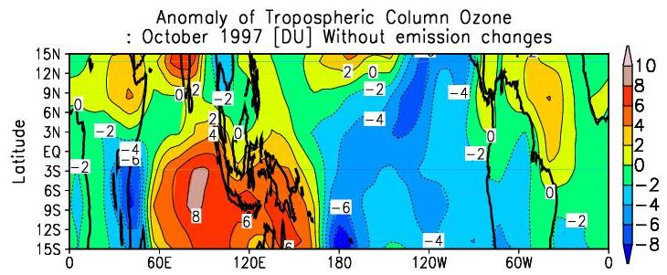
We conducted a simulation on the tropospheric ozone change in September and October 1997. Ozone enhancement in Indonesia during this period was reported in Fujiwara et al.,[1997], and elevated CO levels over Indonesia were also observed(Sawa et al., 1999). Satellite derived data from EP TOMS (Chandra et al., 1998) also indicates these changes(Figure 4).
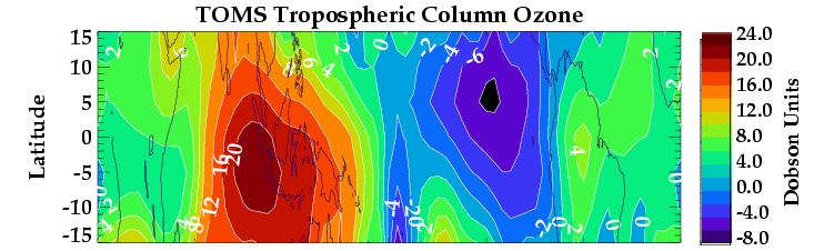
Figure 4. EP TOMS CCD TCO (DU) anomaly of Oct. 1997 minus Oct. 1996 (Chandra et al., 1998).
In addition to the extensive forest fire event occurred in Indonesia, Meteorological changes in convection, humidity, precipitation, and transport from the stratosphere cold be big contributors to observed ozone change. In this simulation, SST data and ECMWF wind and temperature data of 1996, 1997 were used as nudging input to the GCM for a direct comparison to Chandra et al.,1998. Emission change due to extensive forest fire in Indonesia is not included in order to evaluate the effect of meteorological changes itself. Figure 5 shows simulated TCO(Tropospheric Column Ozone) anomaly corresponding to Figure 4. An asymmetrical dipole centered near the date line with TCO is well reproduced. It should be noted that simulated TCO enhancement in Indonesia is underestimated just because emission change associated with the extensive forest fire in Indonesia is not considered in this simulation.

Figure 5. Simulated TCO anomaly with no emission change (corresponding
to Figure 7).
Figure 6 shows the simulated difference of specific humidity (g/kg), ozone chemical lifetime change rate (%) between October 1997 and October 1996. It is clearly seen that chemical life time of ozone over Indonesian region is 2 or 3 times longer in October 1997 than in October 1996. This is just correspondig to much drier condition in Indonesia.
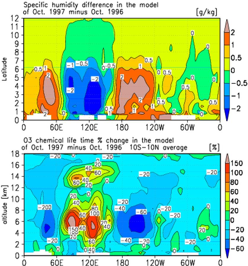
Figure 6. Differences of specific humidity (g/kg) and change rate of ozone
chemical life time (%) between October 1997 and October 1996 in
10S-10N.
Figure 7 shows ozone concentration (ppbv) which originates in the stratosphere over Indonesian region for October 1997 and October of climatological run of the model. It is clear that more ozone intruded to the lower latitude from the mid latitude in both hemisphere in October 1997 compared to the climatological condition. This could be associated with low convective activity and low humidity in the Indonesian region during this period. These changes in humidity, convection and transport of stratospheric ozone consequently caused the tropospheric ozone change seen in Figure 5.
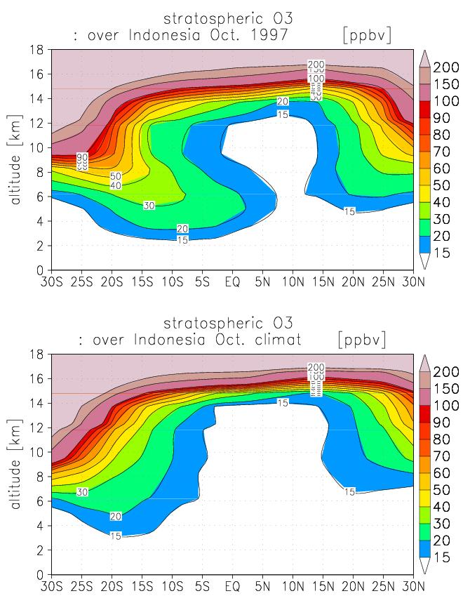
Figure 7. Zonal averaged ozone concentration from the stratosphere over
Indonesia. (ppbv) upper;1997, lower; climatological
References
Chandra, S., J.R..Ziemke, W.Min and W.G. Read, Effects of 1997-1998
El Nino on tropospheric ozone and water vapor, Geophys. Res. Lett., 25, 3867-3870, 1998.
Fujiwara, M., K. Kita, S. Kawakami, T. Ogawa, N. Komala, S. Saraspriya,
and A. Suripto, Tropospheric ozone enhancements during the Indonesian
forest fire events in 1994 and in 1997 as revealed by ground-based
observations, Geophys. Res. Lett., 26 , 2417-2420, 1999.
Olivier, J.G.J., Bouwman, A.F., Van der Maas, C.W.M., Berdowski,
J.J.M, Veldt, C. Bloos, J.P.J., Visschedijk, A.J.H., Zandveld,
P.Y.J., Haverlag, J.L, Description of EDGAR Version 2.0. A set
of global emission inventories of greenhouse gases and ozone-depleting
substances for all anthropogenic and most natural sources on a
per country basis and on 1ox1o grid. RIVM/TNO report, December
1996. RIVM, Bilthoven, RIVM report nr. 771060 002. [TNO MEP report
nr. R96/119], 1996.
Sawa, Y., H. Matsueda, Y. Tsutsumi, J. B. Jensen, H. Y. Inoue,
and Y. Makino, Tropospheric carbon monoxide and hydrogen measurements
over Kalimantan in Indonesia and northern Australia during October,
1997, Geoph. Res. Lett., 26 , 1389-1392, 1999.
Back to
| Session 1 : Stratospheric Processes and their Role in Climate | Session 2 : Stratospheric Indicators of Climate Change |
| Session 3 : Modelling and Diagnosis of Stratospheric Effects on Climate | Session 4 : UV Observations and Modelling |
| AuthorData | |
| Home Page | |