Previous: Total ozone amounts and trends Next: Water vapour trends Up: Ext. Abst.
4. Temperature trends
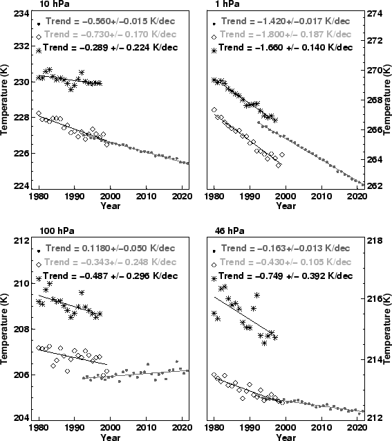
The annual mean model temperature trends are shown in Fig. 6 in comparison with trends determined from Stratospheric Sounding Unit (SSU)/Microwave Sounding Unit (MSU) data (Scaife et al., 2000a) for the slightly shorter period Jan 1980 - Dec 1997. The solar cycle has been removed from the observations (see e.g. Scaife et al., 2000a), but other processes such as the quasi-biennial oscillation and the impacts of aerosol have not been accounted for. In the upper stratosphere the model is broadly in agreement with observations but diverges from them both in the mesosphere and in the middle and lower stratosphere. The temperature trends are to a first approximation independent of latitude. Significant deviations from this occur in the lower stratosphere in southern middle latitudes where the 0.0 and -0.25 contours buckle upwards. The feature is absent in the observations but its cause in the model may be related directly to the ozone trend which also shows an increase in that region. Over Antarctica, where the SSU trends are less reliable, the observations indicate the cooling occurs in the lower stratosphere due to the ozone hole and this is followed by an upper region of warming. Qualitatively, this also occurs in the model, but the influence of the ozone hole does not extend as far north as indicated in the SSU/MSU data.
A quantitative comparison of the globally and annually averaged
temperature trends at selected levels (Fig. 7) confirms many of
these points. In the figure, comparisons are also made with our
previous results from a model without coupled chemistry (Butchart
et al., 2000, small circles). Although this simulation covered
a different period (1992 to 2051), the changes in GHG amounts
and sea conditions were approximately linear throughout the period
and changed at virtually the same rate as for the period studied
here (1980-2000). Thus the Butchart et al. (2000) simulation provides
an important benchmark for model comparisons. The inclusion of
(model computed) ozone trends increases model cooling rates significantly
throughout the stratosphere, in agreement with Langematz (2000)
and Rosier and Shine (2000). This leads to better agreement with
observations in the lower stratosphere (indicated by the results
for 46 and 100 hPa). In the middle stratosphere, the modelled
trends are significantly larger than observed and inclusion of
ozone results in poorer agreement with observations. In the upper
stratosphere, the previous underprediction of observed trends
is replaced by a slight overprediction (within the error bars).
In the Figure the quoted error bars (2![]() ) are the errors in determining the trend from the sequence of
annual temperatures, and in the case of the observations do not
include any error due to removal of the solar cycle or instrument
drift.
) are the errors in determining the trend from the sequence of
annual temperatures, and in the case of the observations do not
include any error due to removal of the solar cycle or instrument
drift.
 |
Previous: Total ozone amounts and trends Next: Water vapour trends Up: Ext. Abst.