Lunar and Planetary Laboratory, University of Arizona, Tucson
AZ 85721-0092, USA.
FIGURES
Abstract
Introduction
A quantitative understanding of the influence of solar ul- traviolet variability on the stratosphere-troposphere system re- quires both observations of the atmospheric response and the development of detailed physical models that explain that re- sponse. On the time scale of the 27-day solar rotation pe- riod, such an understanding has been partially achieved, at least in the case of the observed response of ozone at low latitudes [1,2]. However, on the time scale of the 11-year solar cycle, there are large differences between the observed stratospheric response and that which is predicted by existing models. Some of this difference may be a result of measure- ment inaccuracies; however, a significant part of the difference appears to be a result of model deficiencies. In this paper, the observed characteristics of the 11-year stratospheric response are first summarized, based mainly on satellite measurements of stratospheric temperature and ozone. Emphasis is placed on annually averaged measurements at low to middle latitudes. Comparisons are made with the predictions of a current gen- eral circulation model [3] to illustrate the differences between available models and observations. Possible mechanisms for explaining these differences are then discussed.
Observations and Model Comparisons
Observational evidence for a quasi-decadal oscillation (QDO) of the lower stratosphere and upper troposphere that is approx- imately in phase with the 11-year solar cycle has previously been reported using both long-term meteorological data [4,5] and column ozone data [6,7,8]. At high latitudes in winter, it has been found necessary to separate the data according to the phase of the equatorial quasi-biennial wind oscillation (QBO) in order to demonstrate a correlation between lower strato- spheric meteorological parameters and solar UV proxies such as the 10.7 cm radio flux (e.g., ref. [4]). At low latitudes (! 50 ffi), no such division of the data according to QBO phase is necessary to investigate a possible solar response although the QBO is still a major source of interannual variability.
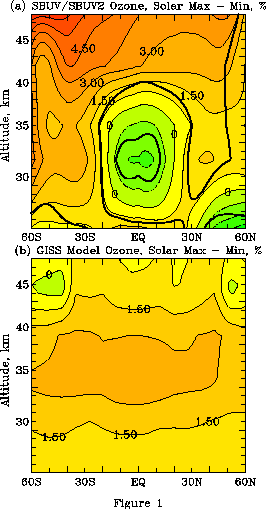
Evidence for an apparent , 11-year variation of upper stratospheric ozone, temperature, and zonal wind has previ- ously been reported based on satellite data sets extending over a minimum of one solar cycle [9,10,11,12]. Based mainly on Nimbus 7 SBUV ozone profile data, it was found that the observed ozone change from solar minimum to maximum in the 40-50 km altitude range was significantly larger (by about a factor of 2) than the predictions of two-dimensional strato- spheric models. In contrast, the observed change in the mid- dle stratosphere (30-40 km) was significantly less than model predictions. These results have been generally supported by later analyses of SBUV-SBUV/2 data as well as Stratospheric Aerosol and Gas Experiment (SAGE) I/II data extending over 18 years (see Figure 3.5 in SPARC Report No. 1, Assessment of Trends in the Vertical Distribution of Ozone, May, 1998).
Figure 1a shows the annual mean variation of ozone mix- ing ratio (in per
cent) from solar minimum to maximum de- rived from a combination
of Nimbus 7 SBUV and NOAA 11 SBUV/2 data covering a 16-year period
(1979-1994). A mul- tiple regression statistical model including
linear trend, QBO, and volcanic aerosol terms in addition to the
solar term was applied to the data following the method of McCormack
and Hood [13], The heavy dark line separates regions where so-
lar regression coefficients are statistically significant at the
2oe level from regions where no significant solar variation could
be measured. The largest variation of more than 3% is present
in the upper stratosphere at altitudes greater than 45 km while
the solar variation in the tropical middle stratosphere is not
statistically significant. Figure 1b shows the ozone variation
from solar minimum to maximum predicted by a representa- tive
general circulation model with parameterized chemistry [3] (D.
Shindell, priv. comm., 2000). The model ozone varia- tion reaches
a maximum of , 2.5% in the middle stratosphere (30-40 km altitude).
Although early estimates of the solar cycle variation of temperature in the middle and upper stratosphere relied on NCEP Climate Prediction Center (CPC) data derived from measurements by the Stratospheric Sounding Units (SSU) on the NOAA operational satellites, these estimates are subject to errors introduced by satellite changes. As discussed in the 1998 WMO Assessment report [ref. 14, p. 5.30], adjustments to the SSU time series using overlap periods allow an improved combined data set to be constructed covering the 1979-1995 period (17 years).
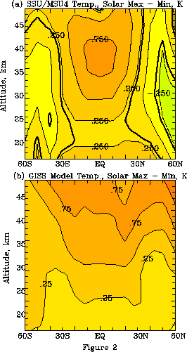
Figure 2a shows the mean stratospheric temperature vari- ation from solar minimum to maximum as derived from the overlap adjusted SSU data by the SPARC Stratospheric Tem- perature Trends Assessment project. At the lower boundary, estimates are based on measurements with Channel 4 of the Microwave Sounding Units (MSU) on the TIROS-N NOAA operational satellites [15]. The heavy dark lines separate re- gions where regression coefficients were positive at the 95% confidence level from regions where the coefficients were not significantly different from zero. A maximum temperature variation of , 0.8 K is present near 40 km altitude in the tropics. The amplitude decreases with decreasing altitude but begins to increase again in the tropical lowermost stratosphere. Figure 2b shows annual mean temperature changes from so- lar minimum to maximum estimated with the GISS GCM (D. Shindell, priv. comm.). Maximum temperature changes oc- cur in the upper stratosphere and decrease continuously with decreasing altitude. No increase in amplitude occurs in the lowermost stratosphere.
In order to assess further the possible existence of a sig- nificant solar cycle variation in lower stratospheric temper- The Solar Component of Stratospheric Variability: Hood and Soukharev ature, we consider further the MSU Channel 4 temperature record noted above. Channel 4 of the MSU instrument yields brightness temperature measurements at a series of frequen- cies near the 60-GHz oxygen absorption band. These represent weighted mean atmospheric temperatures in a layer with peak power at 75 hPa and half-power at 40 and 120 hPa [15]. This pressure range is mainly in the lowermost stratosphere but in- cludes significant contributions from the upper troposphere in the tropics. Standard errors of measurement for 5-day means at individual grid points at 2.5 ffi horizontal resolution are less than 0.25 ffi for most of the globe and less than 0.15ffi for the tropics. These microwave soundings are not affected by the presence of aerosols. Correlations between MSU4 and radiosonde profiles for monthly anomalies are usually above 0.94 and approach unity in some cases. Monthly signal-to-noise ratios are usually over 500 at individual grid points.
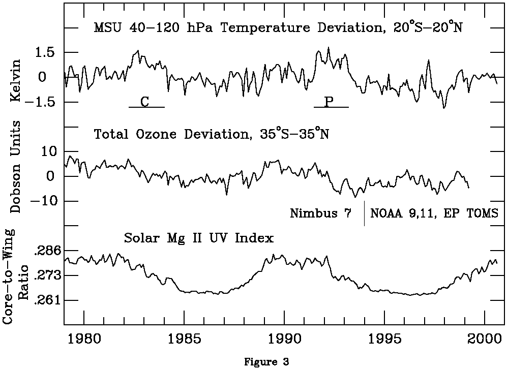
The top panel of Figure 3 shows a simple average of the MSU4 data for the tropics (20 ffi
S to 20ffi N) but with the equatorial data removed to minimize
interannual variability associated with the QBO. In addition to
positive temperature anomalies resulting from the El Chichon (C)
and Pinatubo (P) volcanic aerosol injection events, a long-term,
approximately decadal variation is also present. As indicated
in the lower panel of Figure 3, this decadal variation is roughly
in phase with the Mg II index, a satellite-based proxy for solar
UV variations. (The Mg II data are based on Nimbus 7 SBUV measurements
prior to January, 1994 and on UARS SUSIM measurements afterwards.)
Specifically, ignoring the periods following major volcanic eruptions,
the mean temperature de- viation during solar minima is 0.5-0.8
K lower than during solar maxima. (Application of a multiple regression
statisti- cal model yields an estimated solar cycle variation
of 0.70 \Sigma 0.18 K.) During the past several years as the solar
UV flux has increased toward the next solar maximum, the mean
tropical temperature has also increased significantly by more
than 0.5 K. An increase of similar magnitude occurred between
1986 and the 1990 solar maximum. These temperature increases can
not be attributed easily to volcanic influences and are most probably
solar in origin.
In order to investigate whether a significant variation of ozone
from solar minimum to maximum is present in the lowermost stratosphere,
we consider here a column ozone record derived from a combination
of Total Ozone Mapping Spectrometer (TOMS) data and measurements
by the Solar Backscattered Ultraviolet (SBUV) instruments on the
Nimbus 7, NOAA 9, NOAA 11, Meteor 3, and Earth Probe satellites
[16]. A merged record covering the period from January 1979 through
December 1998 (R. Stolarski, private communication, 1999) was
specifically studied. The second panel of Figure 3 shows a tropical
average of the merged record. The intercali- bration of the record
is best during the Nimbus 7 period prior to January 1994. In addition
to a long-term trend and possible ozone decreases associated with
the El Chichon and Pinatubo eruptions, a decadal variation is
also evident that is approx- imately in phase with the solar Mg
II record. In particular, an increase in tropical mean ozone occurs
between solar mini- mum in 1986 and solar maximum in 1990 that
can not easily be attributed to volcanic or anthropogenic influences.
Although no evidence for a solar variation is present in the data
after 1994, the shortness of the record (ending in 1998) and remain-
ing questions about instrument intercalibration errors suggest
that these data should not be considered as definitive.
Discussion and Possible Mechanisms
The major areas of disagreement between current model estimates of the stratospheric response to solar variability on the 11-year time scale are: (1) the large differences between the observationally derived ozone response and model predictions in the middle and upper stratosphere; and (2) the evidence for a substantial lower stratospheric response component in both temperature and ozone that is not predicted by available models.
With respect to the upper stratospheric ozone response difference, it should first be noted that ozone at these lev- els is nearly in a state of photochemical equilibrium so that transport effects are less important. Assuming that current model treatments of ozone photochemistry are approximately valid, significant long-term changes in ozone concentration at these levels beyond that expected from solar ultraviolet forc- ing should therefore reflect changes in the concentrations of key trace constituents that determine the ozone catalytic loss rate. Evidence for such changes in the concentrations of up- per stratospheric CH4, NO2, and H2O (all of which indirectly influence the abundance of O3) has been obtained using data from the Halogen Occultation Experiment (HALOE) on the Upper Atmosphere Research Satellite (UARS) [17]. Using a simple photochemical model, Siskind et al. [18] showed that the observed upper stratospheric O3 decrease from 1992 to 1995 (approximately solar maximum to minimum) could be attributed to a combination of (i) decreases in odd oxygen production due to decreased solar flux; (ii) increases in total chlorine; (iii) decreases in CH4 (which affects the abundance of reactive chlorine); and (iv) increases in H2O (which affects the rate of O3 catalytic loss). The solar flux contribution was less than half of that resulting from catalytic loss rate trends.
In principle, long-term variations in tropical upwelling, and
hence in the supply of trace constituents affecting the O3 balance
in the upper stratosphere, may be forced either by vol- canic
aerosol variability or by solar variability, or both. Since increases
in lower stratospheric heating and tropical upwelling occurred
following the injection of Mt. Pinatubo aerosols in 1991, a gradual
decrease in upwelling rate could have occurred from this source
during the 1992 to 1995 period [17]. This could be a potential
cause of the observed decline in upper stratospheric CH4 over
the same period. On the other hand, if significant changes in
lower stratospheric heating occur be- tween solar minimum and
maximum such that the tropical upwelling rate is modified, then
this would be an alternate po- tential cause of the observed CH4
decline. Randel et al. [19] have recently analyzed additional
HALOE data through 1998 to show that the decreasing CH4 concentration
in the upper stratosphere reached an apparent minimum in 1996-1997
and may have begun to increase slightly thereafter. If this rep-
The Solar Component of Stratospheric Variability: Hood and Soukharev
resents, in part, a solar cycle variation of upper stratospheric
CH4, then such a variation would need to be incorporated in existing
models in order to accurately simulate the solar cycle variation
of ozone.
With respect to evidence for a substantial lower strato- spheric component of the 11-year response (e.g., Figure 3), one possibility that is not currently considered in stratospheric models is that the QBO may be modulated slightly by the 11-year solar cycle [20]. Statistical studies of the NCEP equa- torial wind data set demonstrate significant decadal variability of the QBO. However, it is not yet clear that this variability is solar-driven.
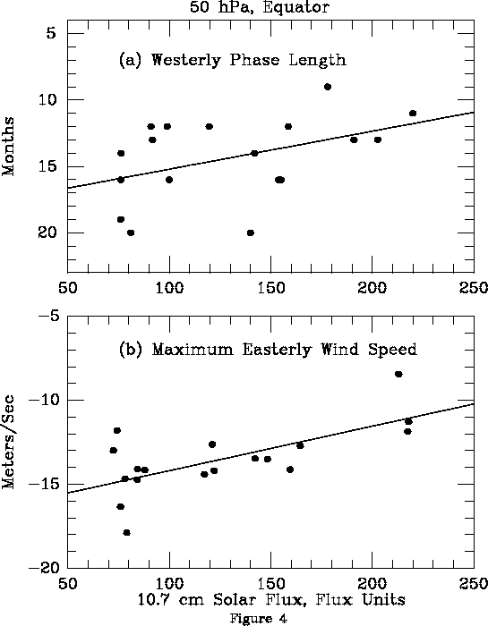
As shown in Figure 4, based on NCEP data for a 40-year period, near the 50 hPa level, some evidence exists for a longer duration of QBO westerlies and a higher amplitude of QBO easterlies under solar minimum conditions. Such a modula- tion would tend to increase the vertical wind shear during the transition to westerlies at levels above 50 hPa, thereby mod- ulating the QBO-induced meridional circulation in the sub- tropics. Specifically, during the transition to westerlies, the induced meridional circulation is characterized by upwelling in the subtropics that reduces the ozone column at these lati- tudes. An increased vertical wind shear under solar minimum conditions would result in deeper ozone minima at these times relative to solar maximum conditions.
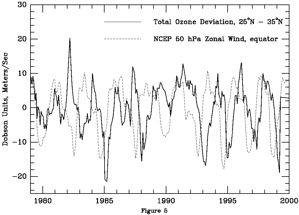
As shown in Figure 5, there is some evidence for such a modulation of the column ozone minima in the northern subtropics. The solid line is the column ozone deviation from the long-term monthly mean while the dashed line is the NCEP 50 hPa zonal wind at the equator. It is seen that deeper ozone minima tend to occur in years when the easterly wind amplitude is larger and the deepest minima tend to occur near solar minima.
However, this possible solar modulation of the QBO- induced meridional
circulation does not easily explain the larger column ozone amounts
in the tropics as a whole at solar maximum as well as the associated
higher tropical mean tem- peratures in the 40-120 hPa layer (middle
panel of Figure 3). A resolution of these issues is required if
general circulation models are to more accurately simulate the
solar component of long-term climate change.
References
(1) Brasseur, G., J. Geophys. Res., 98, p. 23079, 1993
(2) Hood, L. and S. Zhou, J. Geophys. Res., 104, p. 26473, 1999
(3) Shindell, D. et al. Science, 284, p. 305, 1999
(4) Labitzke, K. and H. van Loon, J. Atmos. Terr. Phys., 50, p.
197, 1988
Ann. Geophysicae, 11, p. 1084, 1993; Tellus, 47A, p. 275, 1995
(5) van Loon, H. and D. Shea, Geophys. Res. Lett., 27. p. 2965, 2000
(6) Zerefos, C. W. et al. J. Geophys. Res., 102, p. 1561, 1997
(7) Hood, L., J. Geophys. Res., 102, p. 1355, 1997
(8) Labitzke, K. and H. van Loon, J. Atmos. Terr. Phys., 59, p. 9, 1997
(9) Kodera, K. and K. Yamazaki, J. Meteorol. Soc. Japan, 68, p. 101, 1990
(10) Hood, L. et al., J. Atmos. Sci., 50, p. 3941, 1993
(11) Chandra, S. and R. McPeters, J. Geophys. Res., 99, p. 20665, 1994
(12) McCormack, J. and L. Hood, J. Geophys. Res., 101, p. 20933, 1996
(13) McCormack, J. and L. Hood, Geophys. Res. Lett., 24, p. 2729, 1997
(14) WMO Global Ozone Research and Monitoring Project - Report No. 44, Geneva, Switzerland, 1998
(15) Spencer, R. and J. Christy, J. Climate, 6, p. 1194, 1993;
Spencer et al., J. Climate, 3, p. 1111, 1990
(16) Stolarski, R. et al., Proc. Quad. Ozone Symp., Sapporo 2000,
p. 33, 2000;
DeLand M. et al. Proc. Quad. Ozone Symp., Sapporo 2000,
p. 53, 2000
(17) Nedoluha, G. et al., J. Geophys. Res., 103, p. 3531, 1998;
Geophys. Res. Lett., 25, p. 987, 1998
(18) Siskind, D. E. et al., Geophys. Res. Lett., 25, p. 3513, 1998
(19) Randel, W. J. et al. J. Geophys. Res., 104, p. 3711, 1999
(20) Salby, M. and P. Callaghan, J. Climate, 13, p. 328, 2000.
Back to
| Session 1 : Stratospheric Processes and their Role in Climate | Session 2 : Stratospheric Indicators of Climate Change |
| Session 3 : Modelling and Diagnosis of Stratospheric Effects on Climate | Session 4 : UV Observations and Modelling |
| AuthorData | |
| Home Page | |